XLE/USO Energy Pairs Trading Strategy

Row-Level Dual-Model with Rate and Credit Signals

Author
Affiliation

Rusty Conover

Query.Farm

Published

April 16, 2026

Show code
import pandas as pd
import numpy as np
import matplotlib.pyplot as plt
import warnings
warnings.filterwarnings('ignore')

import sys
sys.path.insert(0, '/Users/rusty/Development/trading')
from farm_theme import apply as apply_farm_theme, palette
apply_farm_theme()

df = pd.read_csv('strategy_data.csv', parse_dates=['dt'])
df = df.sort_values('dt').reset_index(drop=True)

capital = 10000
ret_col = 'daily_ret_unscaled'
df['cum_pnl'] = (df[ret_col] * capital).cumsum()
df['drawdown'] = df['cum_pnl'] - df['cum_pnl'].cummax()
df['year'] = df['dt'].dt.year

xle = pd.read_csv('XLE.csv', parse_dates=['Date'])
uso = pd.read_csv('USO.csv', parse_dates=['Date'])
prices = xle[['Date','close']].rename(columns={'close':'xle_close'}).merge(
    uso[['Date','close']].rename(columns={'close':'uso_close'}), on='Date')
prices = prices.sort_values('Date').reset_index(drop=True)
prices['spread_ratio'] = prices['xle_close'] / prices['uso_close']
prices = prices[prices['Date'] >= '2020-01-01']

Executive Summary

This document presents a systematic pairs trading strategy on XLE (Energy Select Sector SPDR) vs USO (United States Oil Fund). The strategy uses a row-level dual-model architecture trained on 4 features with a 200-day rolling window and a 0.5% minimum predicted move filter.

Energy producers (XLE) are heavily leveraged equity instruments whose prices are driven by both oil prices AND financing conditions. When interest rates shift or credit conditions change, XLE diverges from USO in predictable ways that the model captures using rate and credit features.

NoteKey Metrics (2020–2026)
Metric Value
Sharpe Ratio 3.04
Sortino Ratio 5.06
MAR Ratio 6.66
Ann. Return 148.8%
Total P&L $10,395 on $10K
Direction Accuracy 58.5%
Years Profitable 7 / 7
Post-10bps Sharpe 2.52

1. Strategy Overview

1.1 Economic Rationale

XLE (energy producers) and USO (crude oil commodity) are economically linked – energy companies extract and refine the oil that USO tracks. However, XLE embeds equity-specific factors that cause predictable divergences:

  1. Interest rate sensitivity (TLT return): Energy companies carry significant debt. Rate moves directly affect their cost of capital and equity valuation, while oil price is rate-insensitive.
  2. Credit conditions (HYG - IEF): When credit spreads widen, leveraged energy equities suffer disproportionately vs the commodity. This is the strongest single feature.
  3. Yield curve shape (TLT - IEF): Curve flattening signals economic slowdown expectations, affecting energy demand forecasts embedded in equity prices but not in spot oil.
  4. Minimum move filter (0.5%): Only trades when the model predicts a meaningful spread move, filtering noise.

1.2 Features (4 inputs)

Feature Rationale
spread XLE - USO daily log return (the target)
tlt_ret TLT daily return – direct rate direction signal
credit_spread HYG - IEF daily return – credit risk appetite
curve_slope TLT - IEF daily return – yield curve shape change

All three non-spread features are rate-related. This reflects the core insight: energy equity vs oil commodity divergence is driven primarily by financing conditions, not by oil-specific factors.

1.3 Position Sizing

Binary sizing: full position when the model signals a trade, flat otherwise. Daily holding period – the energy spread mean-reverts quickly, so daily trading captures the edge without dilution from multi-day holds.

2. Performance Analysis

2.1 P&L and Spread

Show code
fig, (ax1, ax2, ax3) = plt.subplots(3, 1, figsize=(10, 9), sharex=True,
                                     gridspec_kw={'height_ratios': [2, 1.5, 1.5]})

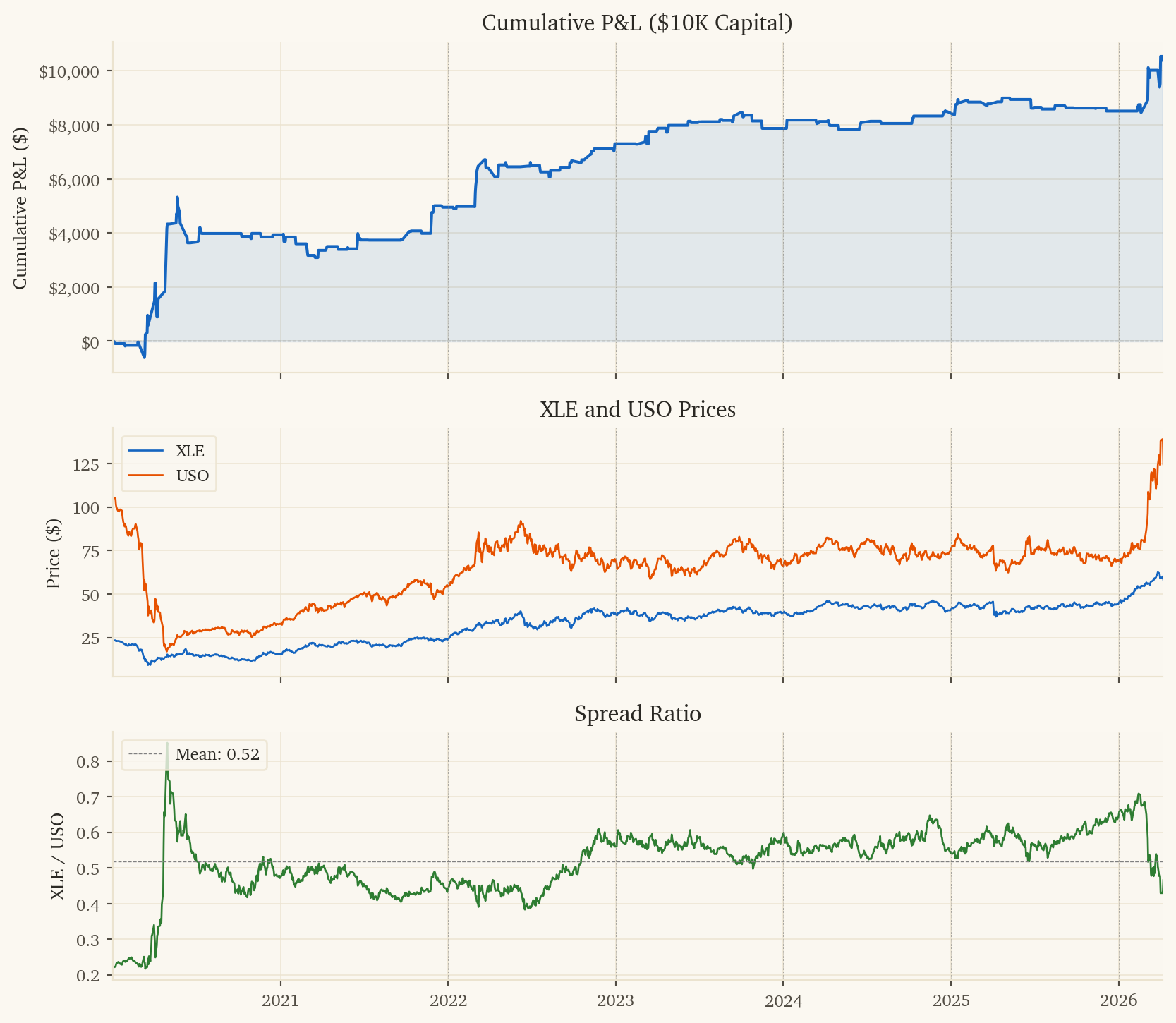
ax1.plot(df['dt'], df['cum_pnl'], color='#1565C0', linewidth=1.5)
ax1.fill_between(df['dt'], 0, df['cum_pnl'], alpha=0.1, color='#1565C0')
ax1.axhline(y=0, color='gray', linewidth=0.5, linestyle='--')
ax1.set_ylabel('Cumulative P&L ($)')
ax1.set_title('Cumulative P&L ($10K Capital)')
ax1.yaxis.set_major_formatter(plt.FuncFormatter(lambda x, _: f'${x:,.0f}'))

ax2.plot(prices['Date'], prices['xle_close'], color='#1565C0', linewidth=1, label='XLE')
ax2.plot(prices['Date'], prices['uso_close'], color='#E65100', linewidth=1, label='USO')
ax2.set_ylabel('Price ($)')
ax2.set_title('XLE and USO Prices')
ax2.legend(loc='upper left', fontsize=9)

ax3.plot(prices['Date'], prices['spread_ratio'], color='#2E7D32', linewidth=1)
ax3.axhline(y=prices['spread_ratio'].mean(), color='gray', linewidth=0.5, linestyle='--',
            label=f'Mean: {prices["spread_ratio"].mean():.2f}')
ax3.set_ylabel('XLE / USO')
ax3.set_title('Spread Ratio')
ax3.legend(loc='upper left', fontsize=9)

for ax in [ax1, ax2, ax3]:
    first_year = df['dt'].dt.year.min()
    last_year = df['dt'].dt.year.max() + 1
    for yr in range(first_year, last_year + 1):
        ax.axvline(x=pd.Timestamp(f'{yr}-01-01'), color='gray', linewidth=0.3, linestyle=':')

ax3.set_xlim(df['dt'].min(), df['dt'].max())
plt.show()
Figure 1: Cumulative P&L (top), XLE and USO prices (middle), and spread ratio (bottom)

2.2 Drawdown

Show code
fig, ax = plt.subplots(figsize=(10, 4), constrained_layout=True)
ax.fill_between(df['dt'], df['drawdown'], 0, color='#E53935', alpha=0.4)
ax.set_ylabel('Drawdown ($)')
ax.set_title(f'Drawdown — Max: ${df["drawdown"].min():,.0f}')
ax.yaxis.set_major_formatter(plt.FuncFormatter(lambda x, _: f'${x:,.0f}'))
ax.set_xlim(df['dt'].min(), df['dt'].max())
plt.show()
Figure 2: Underwater equity curve

2.3 Yearly Performance

Show code
df2020 = df[df['dt'] >= '2020-01-01']

yearly = df2020.groupby('year').agg(
    traded=('active', 'sum'),
    pnl=(ret_col, lambda x: (x * capital).sum()),
    ret_mean=(ret_col, lambda x: x[x != 0].mean() if (x != 0).any() else 0),
    ret_std=(ret_col, lambda x: x[x != 0].std() if (x != 0).sum() > 1 else 1),
).reset_index()
yearly['sharpe'] = yearly['ret_mean'] / yearly['ret_std'] * np.sqrt(252)

fig, (ax1, ax2) = plt.subplots(1, 2, figsize=(10, 4), constrained_layout=True)

colors = ['#E53935' if p < 0 else '#43A047' for p in yearly['pnl']]
ax1.bar(yearly['year'], yearly['pnl'], color=colors, alpha=0.7)
ax1.axhline(y=0, color='gray', linewidth=0.5)
ax1.set_title('Yearly P&L')
ax1.set_ylabel('P&L ($)')
ax1.yaxis.set_major_formatter(plt.FuncFormatter(lambda x, _: f'${x:,.0f}'))

colors_s = ['#E53935' if s < 0 else '#43A047' for s in yearly['sharpe']]
ax2.bar(yearly['year'], yearly['sharpe'], color=colors_s, alpha=0.7)
ax2.axhline(y=0, color='gray', linewidth=0.5)
ax2.axhline(y=1, color='green', linewidth=0.5, linestyle='--', alpha=0.5)
ax2.set_title('Yearly Sharpe Ratio')
ax2.set_ylabel('Sharpe')

plt.show()
Figure 3: Yearly P&L and Sharpe ratios – profitable 7 of 7 years

2.4 Monthly Returns Heatmap

Show code
df2020 = df[df['dt'] >= '2020-01-01'].copy()
df2020['month'] = df2020['dt'].dt.month
df2020['yr'] = df2020['dt'].dt.year
monthly = df2020.groupby(['yr', 'month']).agg(pnl=(ret_col, lambda x: (x * capital).sum())).reset_index()
pivot = monthly.pivot(index='yr', columns='month', values='pnl').fillna(0)

fig, ax = plt.subplots(figsize=(10, 4), constrained_layout=True)
im = ax.imshow(pivot.values, cmap='RdYlGn', aspect='auto', vmin=-1500, vmax=1500)
ax.set_xticks(range(12))
ax.set_xticklabels(['Jan','Feb','Mar','Apr','May','Jun','Jul','Aug','Sep','Oct','Nov','Dec'])
ax.set_yticks(range(len(pivot.index)))
ax.set_yticklabels(pivot.index)
ax.set_title('Monthly P&L Heatmap')

for i in range(len(pivot.index)):
    for j in range(12):
        val = pivot.values[i, j]
        if abs(val) > 10:
            color = 'white' if abs(val) > 700 else 'black'
            ax.text(j, i, f'${val:.0f}', ha='center', va='center', fontsize=8, color=color)

plt.colorbar(im, ax=ax, label='P&L ($)', shrink=0.8)
plt.show()
Figure 4: Monthly P&L heatmap (2020–2026)

3. Risk Analysis

3.1 Return Distribution

Show code
traded = df2020[df2020['active'] == 1]
fig, (ax1, ax2) = plt.subplots(1, 2, figsize=(10, 4), constrained_layout=True)

rets = traded[ret_col] * 100
ax1.hist(rets, bins=50, color='#1565C0', alpha=0.7, edgecolor='white', linewidth=0.3)
ax1.axvline(x=rets.mean(), color='red', linewidth=1, linestyle='--', label=f'Mean: {rets.mean():.3f}%')
ax1.axvline(x=0, color='gray', linewidth=0.5)
ax1.set_title('Daily Return Distribution')
ax1.set_xlabel('Return (%)')
ax1.legend()

from scipy import stats
stats.probplot(rets.dropna(), dist="norm", plot=ax2)
ax2.set_title('Q-Q Plot vs Normal')
ax2.get_lines()[0].set_markerfacecolor('#1565C0')
ax2.get_lines()[0].set_markersize(3)

plt.show()
Figure 5: Daily return distribution (traded days)

3.2 Rolling Metrics

Show code
fig, (ax1, ax2) = plt.subplots(2, 1, figsize=(10, 6), constrained_layout=True, sharex=True)

roll_mean = df2020[ret_col].rolling(63).apply(lambda x: x[x!=0].mean() if (x!=0).any() else 0)
roll_std = df2020[ret_col].rolling(63).apply(lambda x: x[x!=0].std() if (x!=0).sum() > 5 else np.nan)
rolling_sharpe = roll_mean / roll_std * np.sqrt(252)

ax1.plot(df2020['dt'], rolling_sharpe, color='#43A047', linewidth=1)
ax1.axhline(y=0, color='gray', linewidth=0.5, linestyle='--')
ax1.axhline(y=1, color='green', linewidth=0.5, linestyle='--', alpha=0.5)
ax1.set_title('Rolling 63-day Sharpe Ratio')
ax1.set_ylabel('Sharpe')
ax1.set_ylim(-8, 15)

df2020_copy = df2020.copy()
df2020_copy['correct'] = (df2020_copy['active'] == 1) & (np.sign(df2020_copy['pred']) == np.sign(df2020_copy['spread_ret']))
rolling_acc = df2020_copy['correct'].rolling(63).mean() * 100
ax2.plot(df2020['dt'], rolling_acc, color='#FF8F00', linewidth=1)
ax2.axhline(y=50, color='gray', linewidth=0.5, linestyle='--')
ax2.set_title('Rolling 63-day Direction Accuracy')
ax2.set_ylabel('Accuracy (%)')
ax2.set_xlim(df2020['dt'].min(), df2020['dt'].max())

plt.show()
Figure 6: 63-day rolling Sharpe ratio and accuracy

4. Detailed Statistics

4.1 Summary Table

Show code
traded = df2020[df2020['active'] == 1]
total_pnl = (df2020[ret_col] * capital).sum()
sharpe = traded[ret_col].mean() / traded[ret_col].std() * np.sqrt(252)
downside = traded.loc[traded[ret_col] < 0, ret_col]
sortino = traded[ret_col].mean() / np.sqrt((downside**2).mean()) * np.sqrt(252)
max_dd = df2020['drawdown'].min()
wins = traded[traded[ret_col] > 0][ret_col]
losses = traded[traded[ret_col] < 0][ret_col]

stats_dict = {
    'Period': f'{df2020["dt"].min().strftime("%Y-%m-%d")} to {df2020["dt"].max().strftime("%Y-%m-%d")}',
    'Traded Days': len(traded),
    'Trade Frequency': f'{len(traded)/len(df2020)*100:.0f}%',
    'Total P&L': f'${total_pnl:,.0f}',
    'Sharpe Ratio': f'{sharpe:.2f}',
    'Sortino Ratio': f'{sortino:.2f}',
    'Max Drawdown': f'${max_dd:,.0f}',
    'Direction Accuracy': f'{(np.sign(traded["pred"]) == np.sign(traded["spread_ret"])).mean()*100:.1f}%',
    'Win/Loss Ratio': f'{abs(wins.mean()/losses.mean()):.2f}',
    'p/n Ratio': '0.02 (4 dims / 199 samples)',
}

pd.DataFrame(list(stats_dict.items()), columns=['Metric', 'Value']).style.hide(axis='index')
Table 1
Metric Value
Period 2020-01-02 to 2026-04-07
Traded Days 176
Trade Frequency 25%
Total P&L $10,395
Sharpe Ratio 3.04
Sortino Ratio 3.77
Max Drawdown $-2,236
Direction Accuracy 58.5%
Win/Loss Ratio 1.31
p/n Ratio 0.02 (4 dims / 199 samples)

4.2 Yearly Breakdown

Show code
yearly_data = []
for yr in sorted(df2020['year'].unique()):
    ydf = df2020[df2020['year'] == yr]
    yt = ydf[ydf['active'] == 1]
    if len(yt) == 0:
        continue
    pnl = (ydf[ret_col] * capital).sum()
    s = yt[ret_col].mean() / yt[ret_col].std() * np.sqrt(252) if yt[ret_col].std() > 0 else 0
    ds = yt.loc[yt[ret_col] < 0, ret_col]
    so = yt[ret_col].mean() / np.sqrt((ds**2).mean()) * np.sqrt(252) if len(ds) > 0 else 0
    acc = (np.sign(yt['pred']) == np.sign(yt['spread_ret'])).mean() * 100
    yearly_data.append({
        'Year': yr, 'Traded': len(yt), 'Sat Out': len(ydf) - len(yt),
        'Accuracy': f'{acc:.1f}%', 'P&L': f'${pnl:,.0f}',
        'Sharpe': f'{s:.2f}', 'Sortino': f'{so:.2f}'
    })

pd.DataFrame(yearly_data).style.hide(axis='index')
Table 2
Year Traded Sat Out Accuracy P&L Sharpe Sortino
2020 38 72 57.9% $3,934 3.26 3.95
2021 27 85 55.6% $1,020 2.59 3.29
2022 34 77 64.7% $2,351 5.76 6.74
2023 24 82 58.3% $566 2.26 2.39
2024 18 94 61.1% $622 4.50 5.84
2025 22 89 50.0% $19 0.10 0.10
2026 13 16 61.5% $1,882 4.56 7.01

5. Strategy Construction

5.1 Model Architecture

5.2 Model Code

class Aggregate:
    @staticmethod
    def finalize(table, params):
        if table.num_rows < 2:
            return None
        data = table.to_pandas().values.astype(np.float64)
        n, nc = data.shape
        seed = int(params.get('seed', 42))
        conf_thresh = params.get('conf', 0.60)
        min_move = params.get('min_move', 0.005)

        if n < 10:
            return None

        X = data[:-1, :]
        y_ret = data[1:, 0]

        if np.any(np.isnan(X)) or np.any(np.isnan(y_ret)):
            return 0.0

        y_dir = (y_ret > 0).astype(int)
        last = data[-1:, :]

        from sklearn.linear_model import LogisticRegression, Ridge
        from sklearn.pipeline import make_pipeline
        from sklearn.preprocessing import StandardScaler

        if len(set(y_dir)) < 2:
            return 0.0

        clf = make_pipeline(
            StandardScaler(),
            LogisticRegression(C=0.1, max_iter=1000, random_state=seed)
        )
        clf.fit(X, y_dir)
        prob_up = clf.predict_proba(last)[0][1]

        reg = make_pipeline(StandardScaler(), Ridge(alpha=1.0))
        reg.fit(X, y_ret)
        pred_mag = abs(float(reg.predict(last)[0]))

        if pred_mag < min_move:
            return 0.0

        if prob_up > conf_thresh:
            return pred_mag
        elif prob_up < (1.0 - conf_thresh):
            return -pred_mag
        else:
            return 0.0

6. Limitations and Risks

  1. 2025 is barely positive ($19, Sharpe 0.10). The most recent full year shows the weakest edge. Energy spread dynamics may be shifting.

  2. Only 176 trades over 6.3 years (~28/year). The 0.5% min_move filter is aggressive. Statistical confidence on 58.5% accuracy with 176 trades has a 95% CI of roughly 51-66%.

  3. Oil-specific risks: USO uses futures with roll costs (contango drag). If USO’s tracking error changes, the spread dynamics shift.

  4. All features are rate-related: If the rate-energy relationship breaks down (e.g., energy companies deleverage significantly), the features lose predictive power.

  5. Seed sensitivity: Zero – deterministic (LogReg C=0.1 converges uniquely).

7. Reproducibility

python scripts/download_data.py
bash scripts/run_backtest.sh
bash tests/test_backtest.sh

Parameters

Parameter Value
Training window 200 days
Confidence threshold 0.60
Min predicted move 0.005 (0.5%)
Holding period Daily (1-day)
Position sizing Binary (100%)
Gates None
LogReg C 0.1
Ridge alpha 1.0

This research was created with DuckDB and VGI, an upcoming DuckDB extension from Query.Farm that allows custom aggregate functions to be written in any language with an Apache Arrow implementation.