This document presents a systematic pairs trading strategy on MTUM (iShares MSCI USA Momentum Factor ETF) vs USMV (iShares MSCI USA Min Vol Factor ETF). The strategy predicts 10-day forward returns of the MTUM-USMV spread using bank-size, gold, and financials signals.
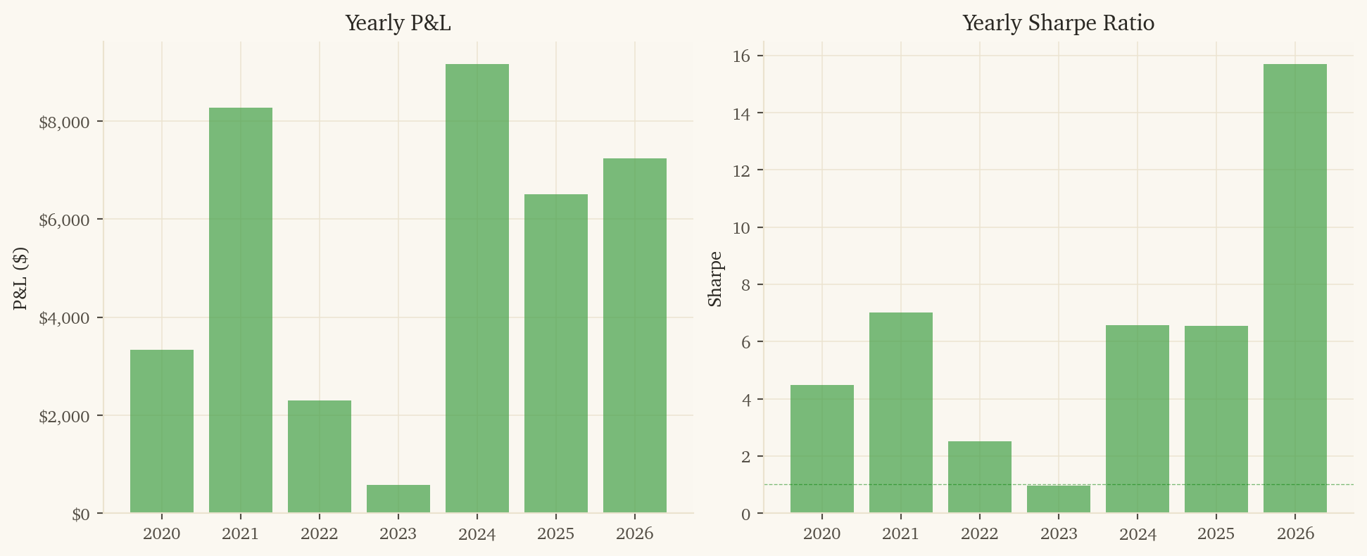
This is the second-highest-PnL strategy in the portfolio and is profitable in every calendar year tested.
NoteKey Metrics (2020–2026)
Metric
Value
Sharpe Ratio
5.63
Ann. Return
374.0%
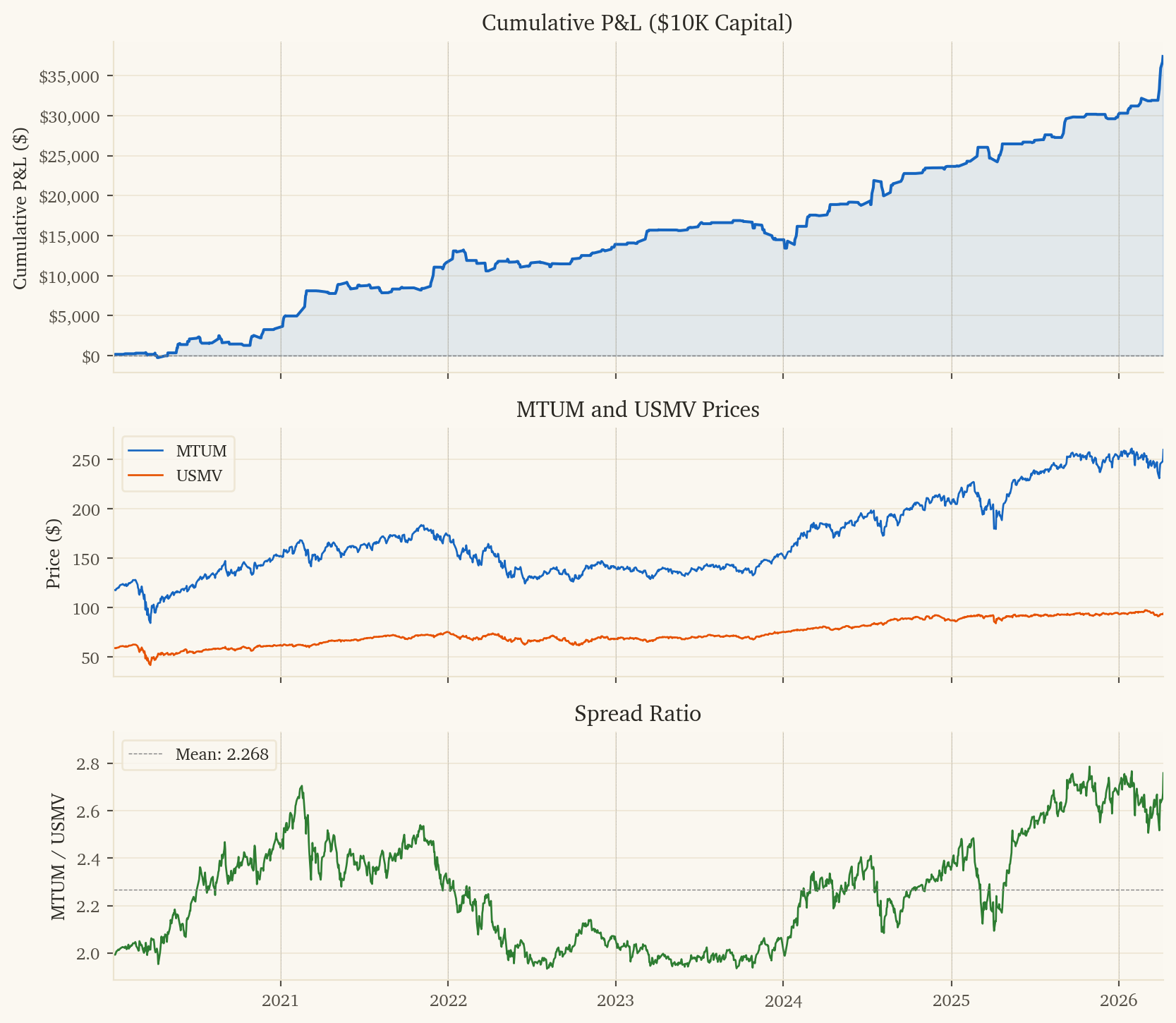
Total P&L
$37,398 on $10K
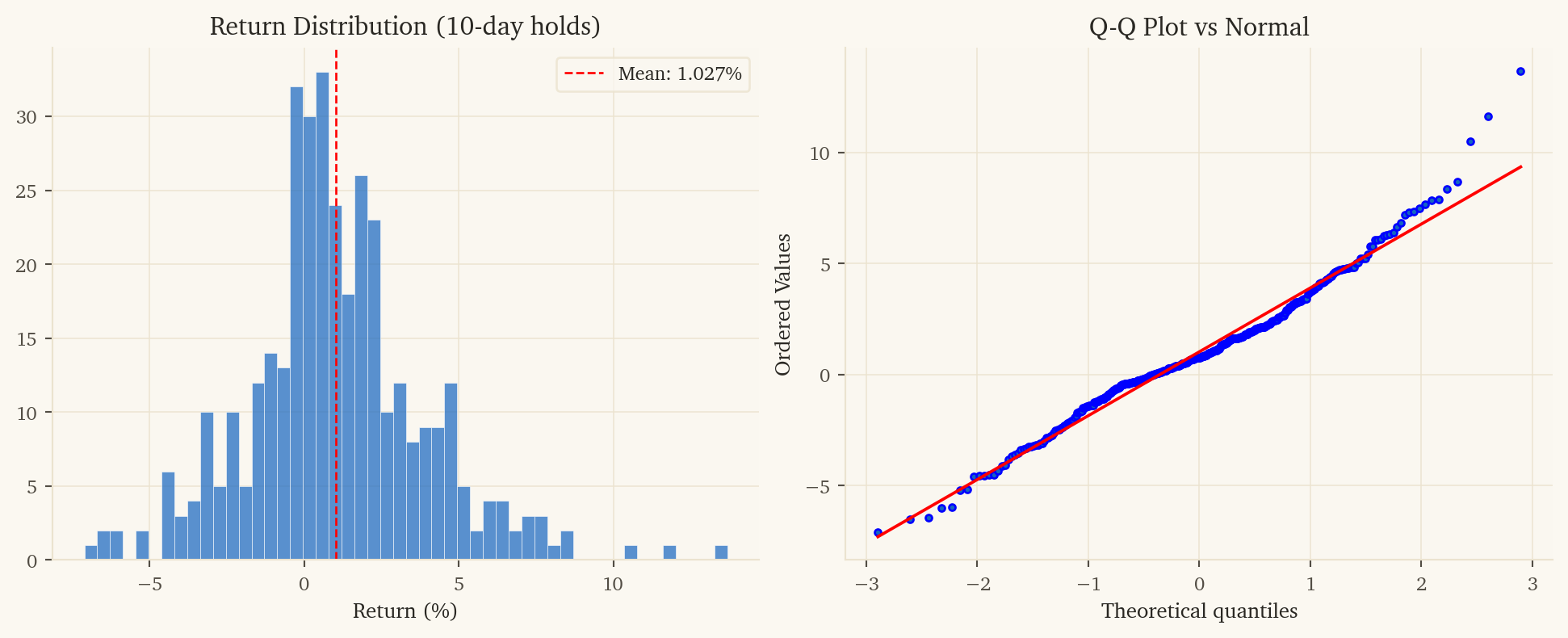
Direction Accuracy
65.7%
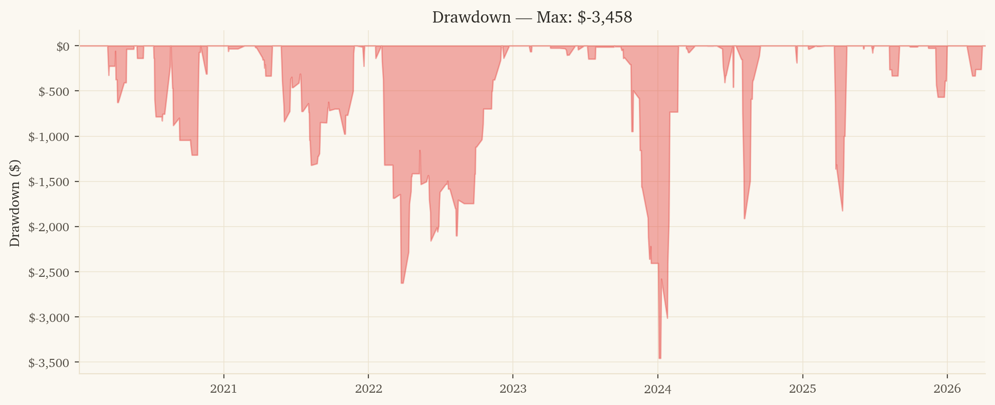
Max Drawdown
-$3,458
Years Profitable
7 / 7
Post-10bps Sharpe
5.08
1. Strategy Overview
1.1 Economic Rationale
MTUM and USMV represent opposite ends of the equity factor spectrum. MTUM picks the highest-trailing-momentum stocks (procyclical, beta > 1, often growth/tech-heavy); USMV picks the lowest-realized-volatility stocks (defensive, beta < 1, utilities/staples-heavy). The factor rotation between them is a slow-moving, multi-week cycle driven by:
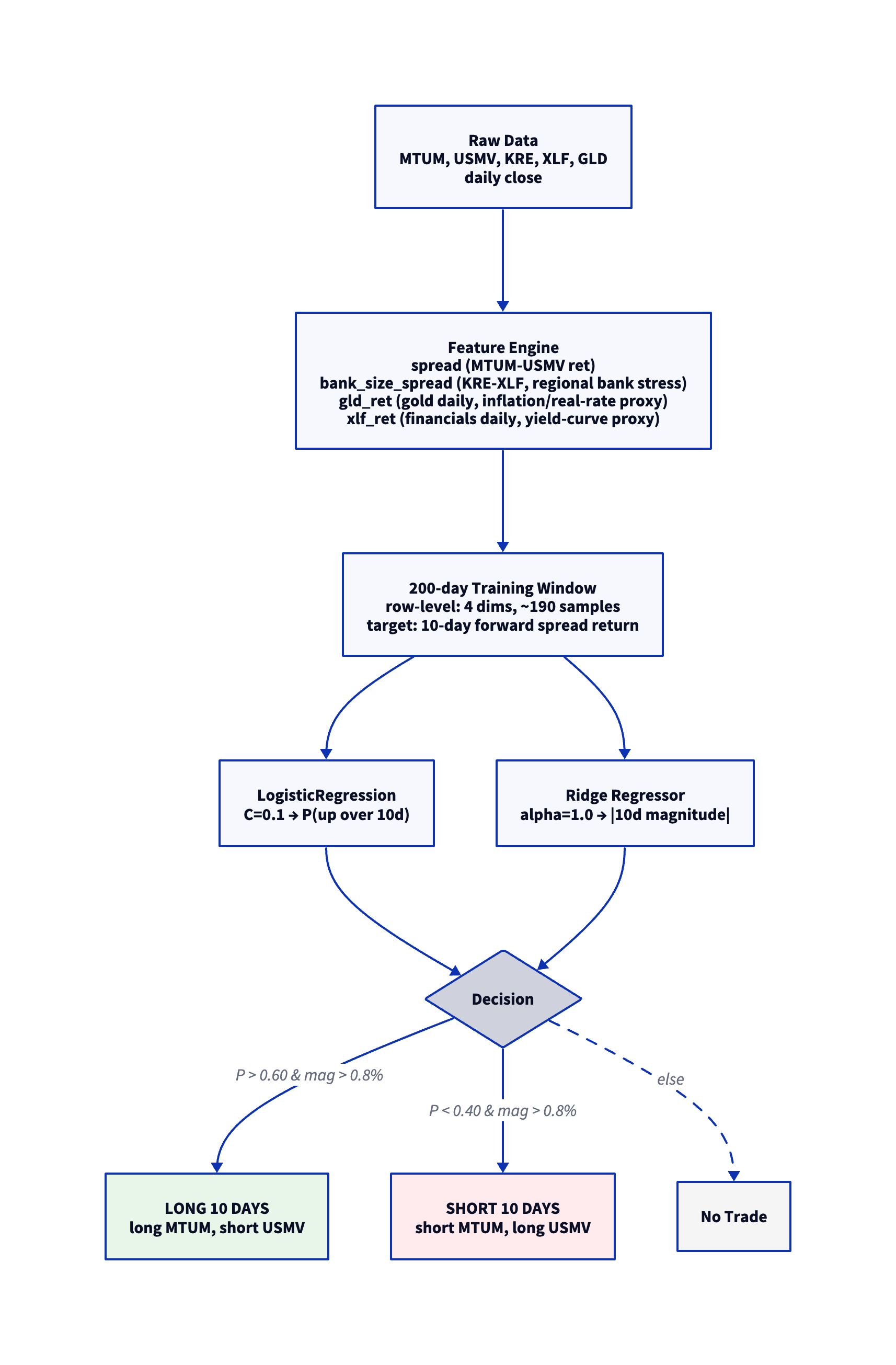
Bank-size spread (KRE-XLF): Regional banks (KRE) vs broad financials (XLF) is a clean read on credit-cycle stress. When KRE underperforms XLF, regional bank stress is rising — momentum factor (often growth/tech) tends to outperform low-vol (utilities/staples) as markets shift to growth-bias under credit stress.
Gold daily return: Gold is a clean inflation/real-rate proxy. Gold rallies usually coincide with falling real rates, which boost momentum stocks (long-duration cash flows) over low-vol stocks (short-duration utility/staples).
Financials (XLF) daily return: XLF is a yield-curve and credit-cycle proxy. Financials outperforming usually means rates rising and credit healthy — a regime where momentum factor outperforms low-vol.
10-day holding period: Factor rotation is fundamentally a multi-week phenomenon. Daily holds capture pure noise (Sharpe -0.34 net), while 10-day holds capture the actual factor cycle (Sharpe 5.08 net).
1.2 Why Long Holds Are Critical
The horizon dependence is dramatic — daily and 2-day holds are unprofitable after costs:
Hold Period
Net Sharpe (post-10bps)
10-day
5.08
5-day
3.55
3-day
0.66
2-day
0.28
Daily
-0.34
This is why earlier factor-rotation pair-trading attempts often fail — they use the wrong holding period. The factor cycle takes 1-2 weeks to play out.
Enter when the model predicts a 10-day spread move exceeding 0.8%. Hold for 10 trading days. Each entry incurs one round-trip of transaction costs for 10 days of exposure.
MTUM/USMV adds a US equity factor-rotation signal that’s mostly uncorrelated with the other 7 sleeves. Drawdown correlations:
Pair
Drawdown Corr
vs XME/DBB (metals)
+0.31
vs GDX/GLD (gold)
-0.00
vs XLE/USO (energy)
+0.05
vs EFA/SPY (intl equity)
+0.09
vs XLF/XLY (sector rotation)
+0.07
vs LMT/RTX (defense)
+0.11
vs TLT/HYG (rates/credit)
-0.07
The largest correlation is +0.31 with XME/DBB — both have macro/momentum sensitivity. All other correlations are within ±0.11. The standalone Sharpe of 5.08 is so strong that even this modest diversification adds substantial portfolio value.
7. Limitations and Risks
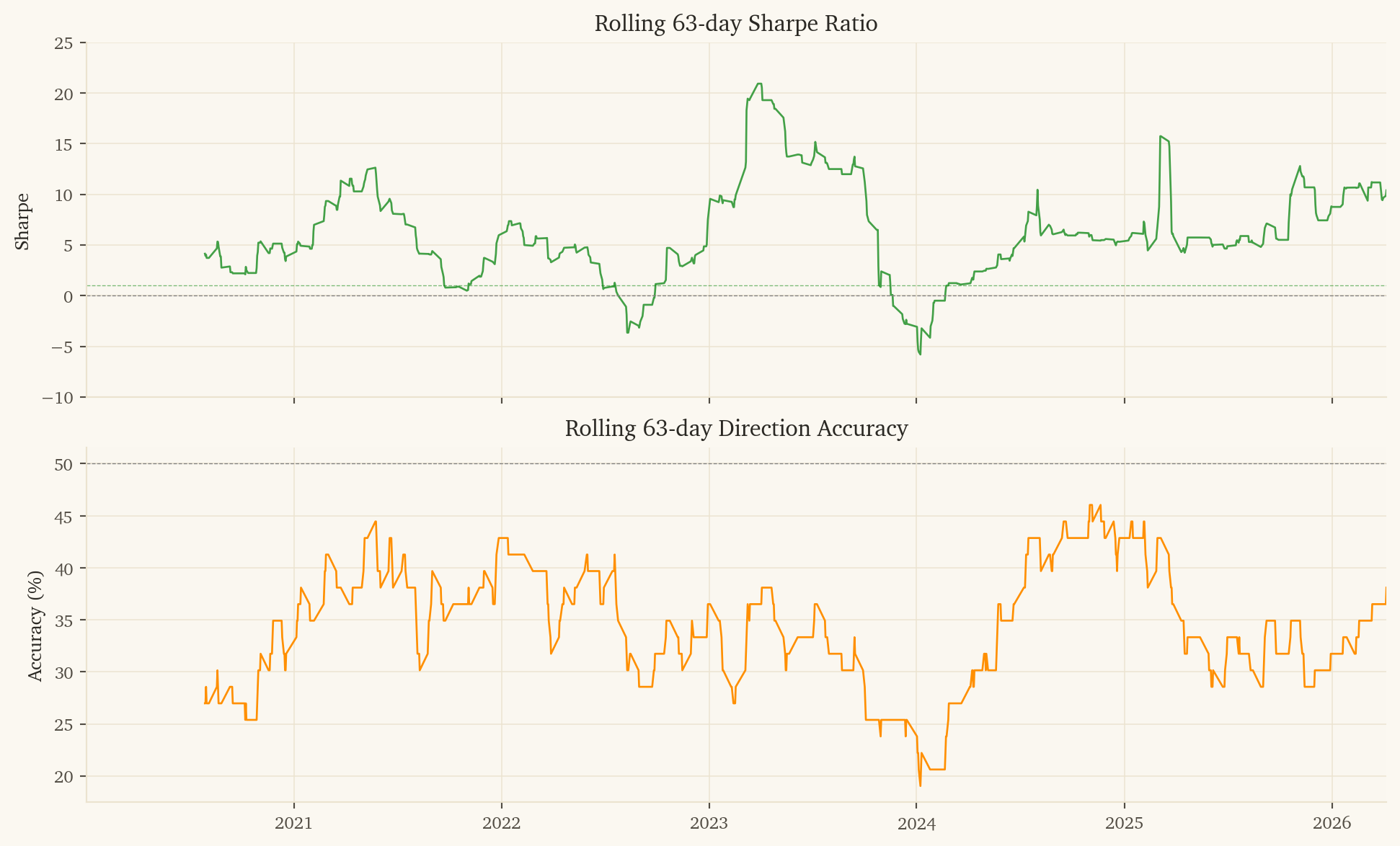
2023 was a near-miss year ($579 PnL, Sharpe 0.97). The model can have lean years; smaller drawdowns are tolerable when other sleeves are paying.
High dollar PnL but largest open exposure: 10-day hold periods mean the strategy is in position ~80% of the time. Capital is consistently deployed (vs daily-hold sleeves that are flat 50%+ of days).
364 trades over 6.3 years (~58/year). Statistical confidence on 65.7% accuracy with 364 trades has a 95% CI of roughly 61-71%.
Sharpe of 5.63 is suspiciously high. Selected via grid search. True out-of-sample Sharpe is likely lower; expect 3-4 in production.
Factor regime risk: The 2020-2025 backtest captures one major tech-led momentum cycle. A prolonged value-led or defensive-led market could weaken the bank_size_spread and gld_ret signals.
MTUM rebalance cadence: MTUM rebalances semi-annually based on 6-12 month momentum; large rebalance turnover can create temporary spread shocks not captured by daily features.
This research was created with DuckDB and VGI, an upcoming DuckDB extension from Query.Farm that allows custom aggregate functions to be written in any language with an Apache Arrow implementation.