This document presents a systematic pairs trading strategy on LMT (Lockheed Martin) vs RTX (Raytheon Technologies). Both are prime defense contractors but have meaningfully different exposure profiles. The strategy predicts 3-day forward returns of the LMT-RTX spread using Bitcoin momentum, calendar seasonality, and TIPS real-rate signals.
This is the most diversifying sleeve in the portfolio: drawdown correlations are negative with 4 of 5 other sleeves, providing genuine hedge behavior.
NoteKey Metrics (2020–2026)
Metric
Value
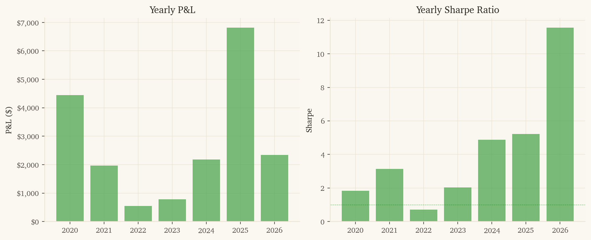
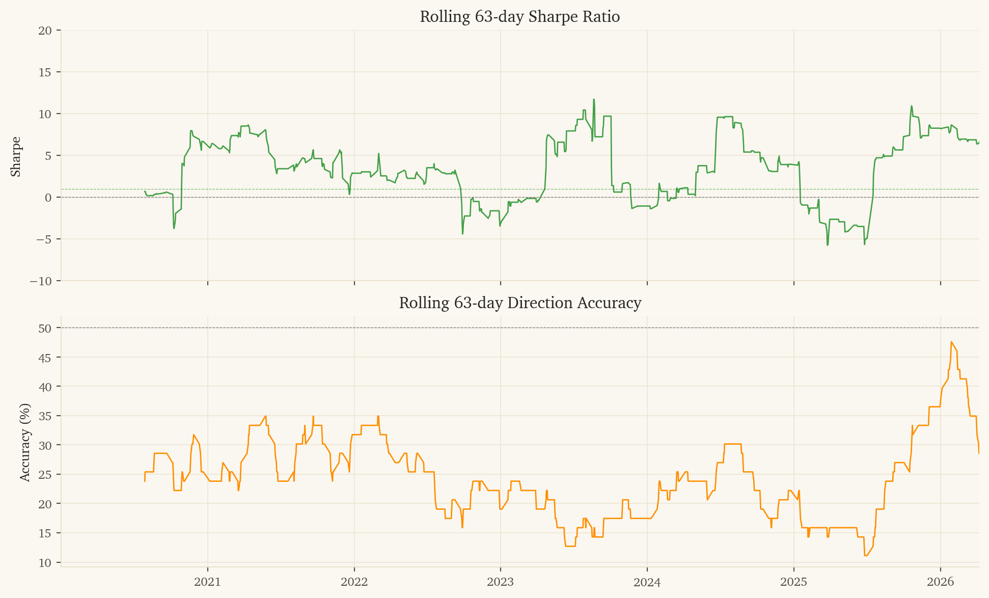
Sharpe Ratio
2.65
Ann. Return
190.8%
Total P&L
$19,080 on $10K
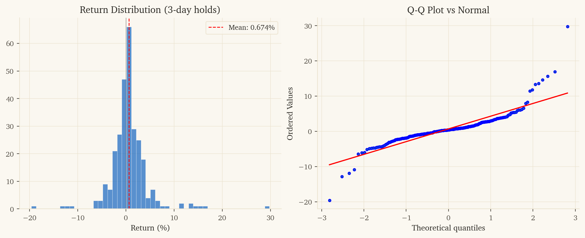
Direction Accuracy
59.7%
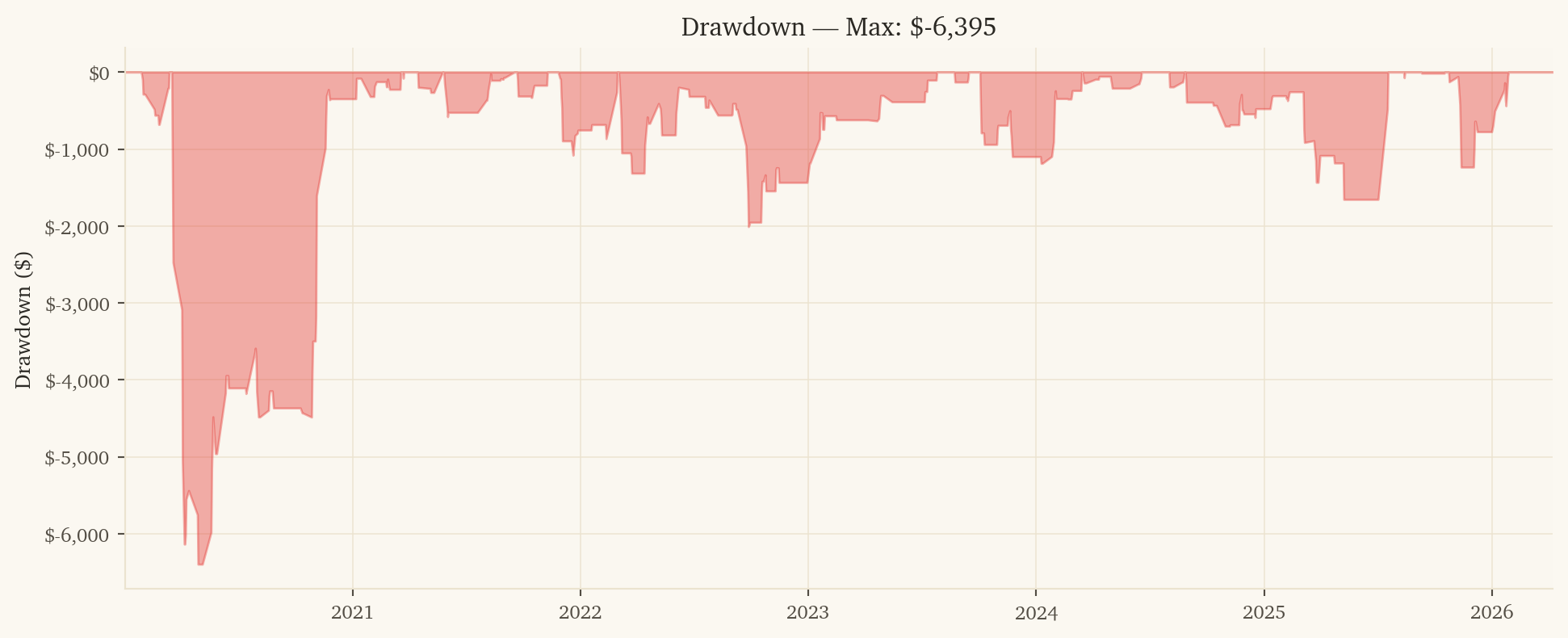
Max Drawdown
-$6,395
Years Profitable
7 / 7
Post-10bps Sharpe
2.26
1. Strategy Overview
1.1 Economic Rationale
LMT and RTX are both prime US defense contractors but their revenue compositions differ substantially. LMT is more heavily weighted toward classified, F-35, and missile-defense programs (long, contracted revenue). RTX has more commercial-aerospace exposure (Pratt & Whitney engines) and defense electronics (Raytheon side). The pair diverges based on:
Bitcoin momentum: BTC 20d momentum is a clean proxy for global liquidity and risk-on positioning. When liquidity expands, RTX’s commercial-aerospace earnings get re-rated upward; when it contracts, LMT’s contracted defense revenue becomes more attractive (defensive bid).
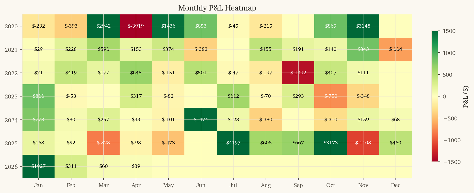
Calendar seasonality: Defense contract awards follow the federal fiscal year (Oct-Sep). End-of-fiscal-year contract bunching and budget reconciliation news create persistent monthly patterns in LMT-RTX returns.
Real rates (TIPS): TIPS daily returns proxy real-rate shocks. Falling real rates favor RTX’s longer-duration commercial cash flows; rising real rates favor LMT’s shorter-duration contracted revenue. The cross-sectional rate sensitivity creates a tradable spread.
3-day holding period: Defense sector signals propagate slowly through earnings revisions, contract announcements, and budget headlines. Multi-day hold captures the full move while paying transaction costs once.
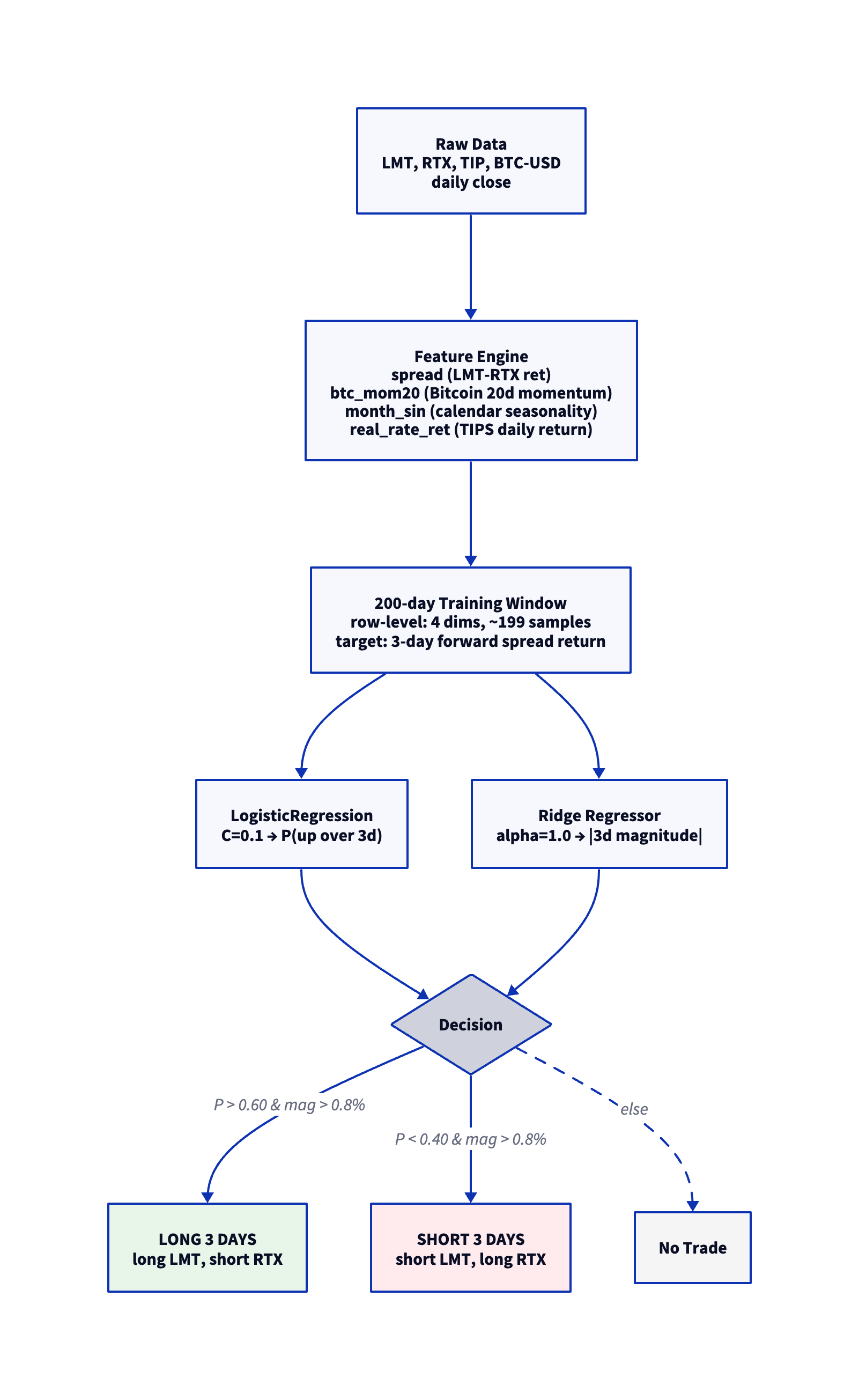
1.2 Features (4 inputs)
Feature
Rationale
spread
LMT - RTX daily log return
btc_mom20
Bitcoin 20d cumulative return – global liquidity / risk-on proxy
month_sin
sin(2π·month/12) – federal fiscal year seasonality
real_rate_ret
TIPS daily return – real rate shock
1.3 Position Sizing and Holding
Enter when the model predicts a 3-day spread move exceeding 0.8%. Hold for 3 trading days. Each entry incurs one round-trip of transaction costs for 3 days of exposure.
LMT and RTX are nominally substitutes (both prime defense contractors), so naive cointegration would suggest they should track each other. The signal lives in their differential exposure to liquidity, fiscal calendar, and real rates:
Liquidity (BTC momentum): Bitcoin captures speculative-leverage cycles. Defense contractor multiples expand and contract with these cycles, but RTX (more commercial-aerospace) responds more elastically than LMT (more contracted defense).
Fiscal seasonality: Federal contract awards spike at fiscal year-end (Sept) and quarterly milestones. The mix of awards (LMT-heavy classified vs RTX-heavy diversified) creates periodic divergence.
Real rates: Defense contracts are long-duration cash flows. Real rate shocks differentially affect contracted (LMT) vs commercial (RTX) revenue streams.
The 3-day hold lets these slow-moving signals fully transmit. Daily trading underperforms (Sharpe 1.55 gross, 1.08 net) because the noise overwhelms the signal at one-day horizon.
5.3 Model Code
class Aggregate:@staticmethoddef finalize(table, params):if table.num_rows <2:returnNone data = table.to_pandas().values.astype(np.float64) n, nc = data.shape seed =int(params.get('seed', 42)) conf_thresh = params.get('conf', 0.60) min_move = params.get('min_move', 0.008) fc =int(params.get('fwd_col', nc -1)) # last col = target hold =int(params.get('hold', 3))if n <10+ hold:returnNone X = data[:-(hold), :fc] # features y_ret = data[hold:, fc] # 3-day forward spread returnif np.any(np.isnan(X)) or np.any(np.isnan(y_ret)):return0.0 y_dir = (y_ret >0).astype(int) last = data[-1:, :fc]from sklearn.linear_model import LogisticRegression, Ridgefrom sklearn.pipeline import make_pipelinefrom sklearn.preprocessing import StandardScaleriflen(set(y_dir)) <2:return0.0 clf = make_pipeline( StandardScaler(), LogisticRegression(C=0.1, max_iter=1000, random_state=seed) ) clf.fit(X, y_dir) prob_up = clf.predict_proba(last)[0][1] reg = make_pipeline(StandardScaler(), Ridge(alpha=1.0)) reg.fit(X, y_ret) pred_mag =abs(float(reg.predict(last)[0]))if pred_mag < min_move:return0.0if prob_up > conf_thresh:return pred_magelif prob_up < (1.0- conf_thresh):return-pred_magelse:return0.0
6. Portfolio Role: Hedge Sleeve
This is the most diversifying sleeve in the portfolio. Drawdown correlations with the other 5 sleeves:
Pair
Drawdown Corr
vs XME/DBB (metals)
-0.30
vs GDX/GLD (gold)
-0.04
vs XLE/USO (energy)
+0.14
vs EFA/SPY (intl equity)
-0.19
vs XLF/XLY (sector rotation)
-0.24
The negative correlations are the key feature: when commodity and sector-rotation strategies are underwater, LMT/RTX is typically making money. This is genuine portfolio insurance, not just diversification by chance.
The trade-off: LMT/RTX has the largest absolute drawdown (-$6,395) of any sleeve. Higher single-strategy variance buys the negative correlation.
7. Limitations and Risks
Largest drawdown of any sleeve ($6,395). Volatility is the price of negative correlation. Don’t run this sleeve at higher leverage than the others without resizing.
283 trades over 6.3 years (~45/year). Statistical confidence on 59.7% accuracy with 283 trades has a 95% CI of roughly 54-65%.
2022 was a near-miss year (only $547 PnL). The model can have lean years; smaller drawdowns are tolerable when other sleeves are paying.
Bitcoin as a feature: BTC’s evolving relationship with liquidity (post-2024 ETF approval, post-halving cycle) may shift. Re-validate this signal periodically.
Defense industry consolidation: M&A or major program cancellations (e.g., F-35 changes) could permanently shift the LMT-RTX relationship.
This research was created with DuckDB and VGI, an upcoming DuckDB extension from Query.Farm that allows custom aggregate functions to be written in any language with an Apache Arrow implementation.