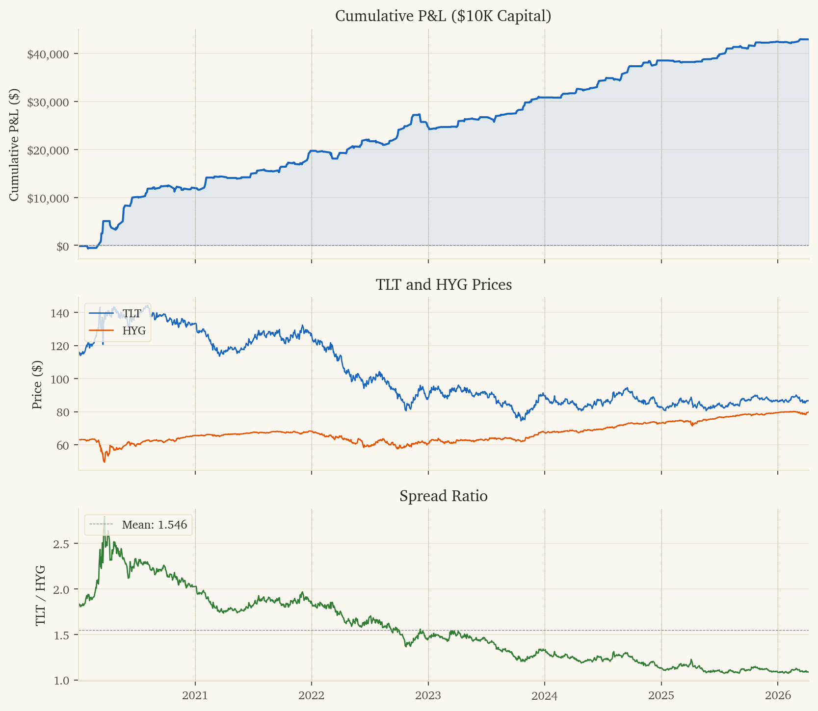
This document presents a systematic pairs trading strategy on TLT (iShares 20+ Year Treasury Bond ETF) vs HYG (iShares iBoxx High-Yield Corporate Bond ETF). The strategy predicts 10-day forward returns of the TLT-HYG spread using credit positioning, mean-reversion, and yield-curve cycle signals.
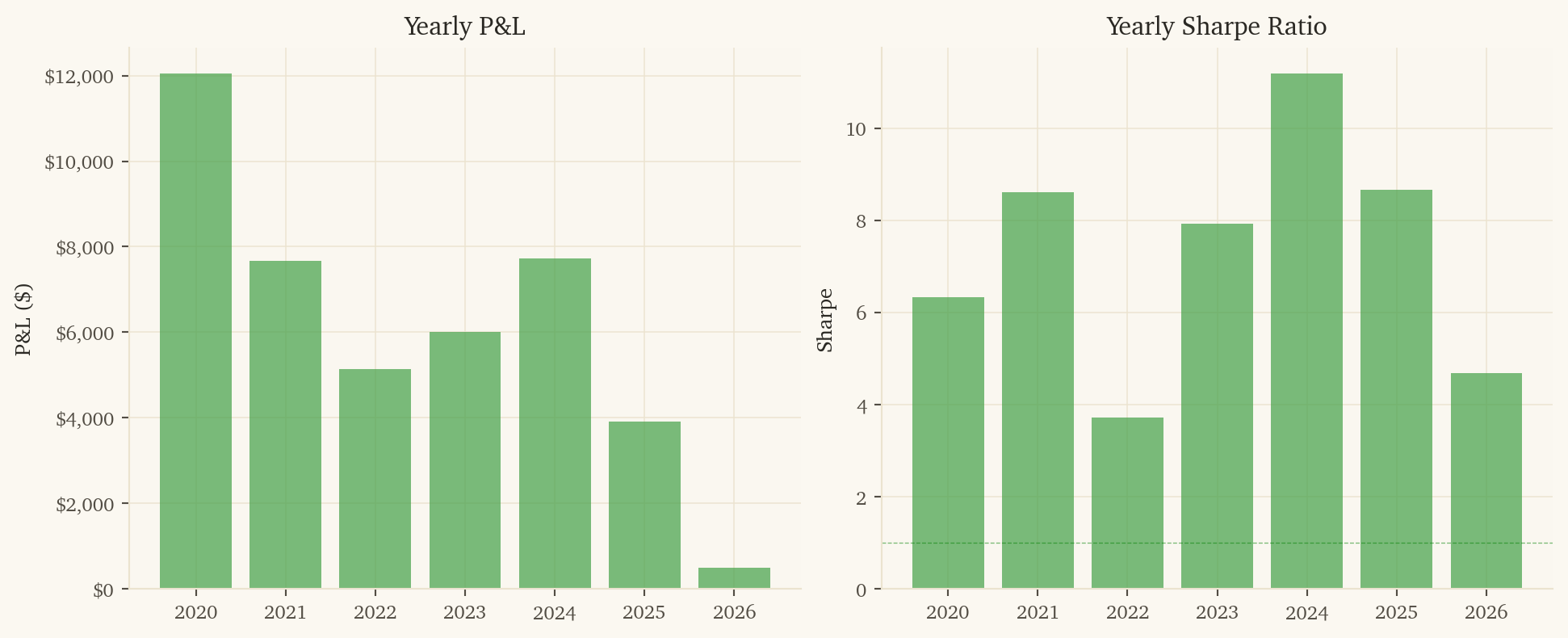
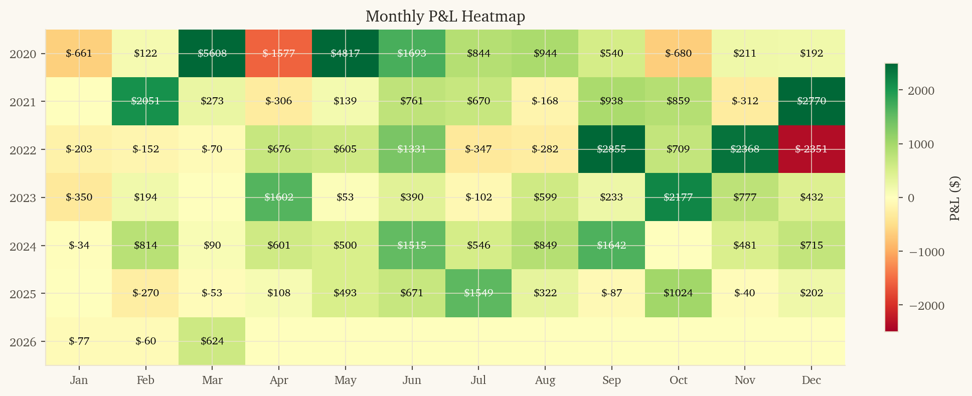
This is the highest-PnL strategy in the portfolio and is profitable in every calendar year tested.
NoteKey Metrics (2020–2026)
Metric
Value
Sharpe Ratio
6.49
Ann. Return
429.9%
Total P&L
$42,987 on $10K
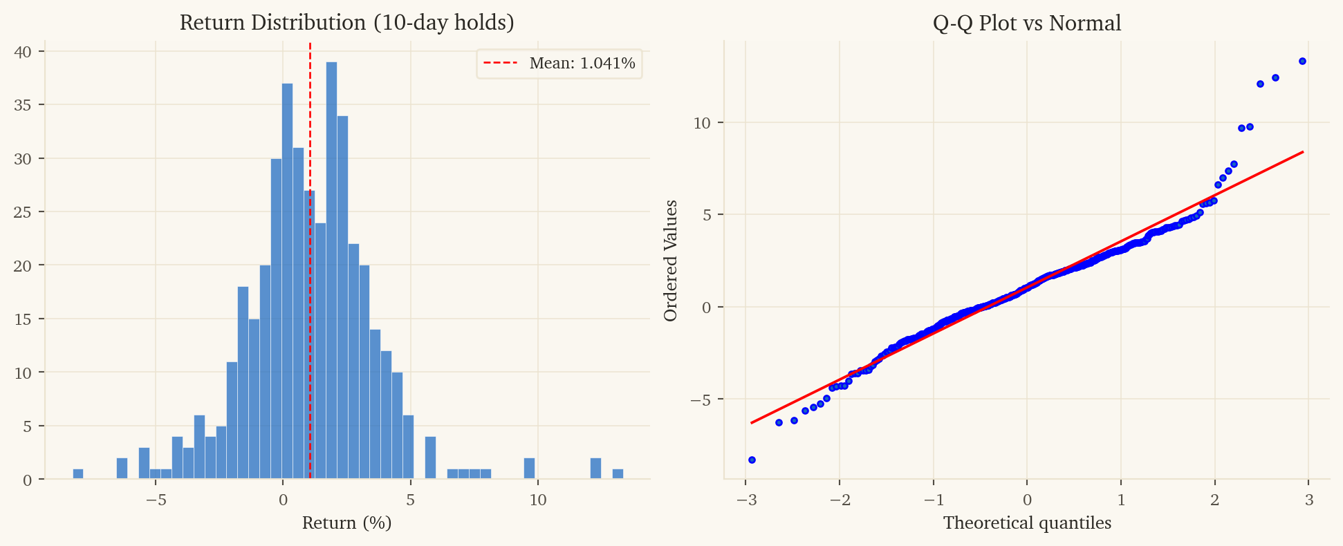
Direction Accuracy
68.0%
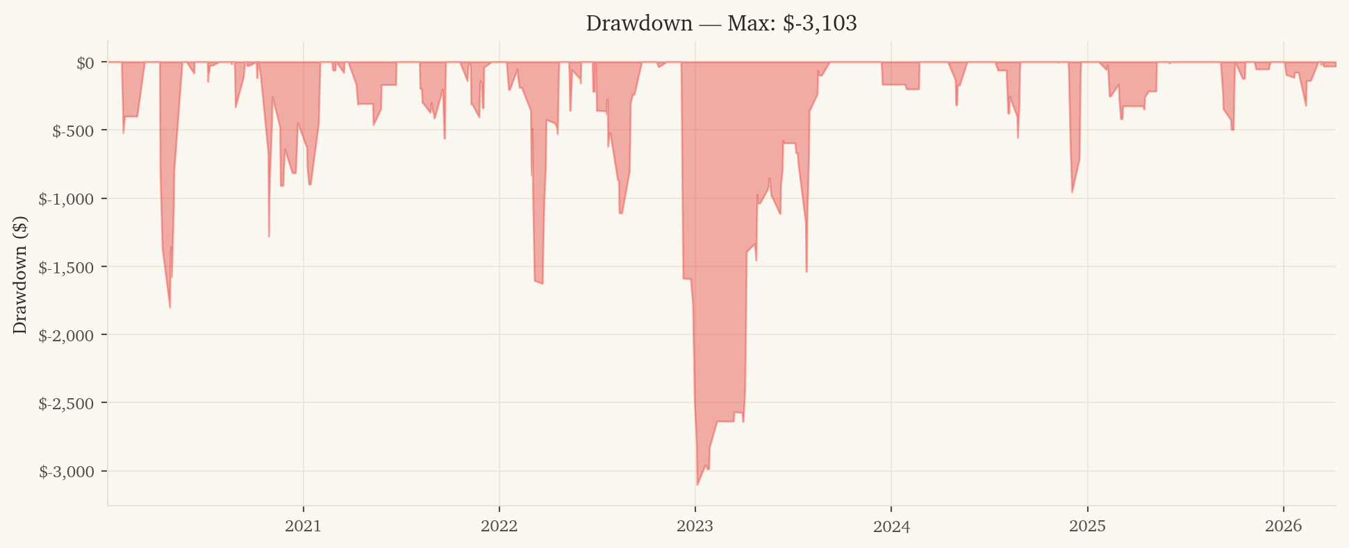
Max Drawdown
-$3,103
Years Profitable
7 / 7
Post-10bps Sharpe
5.86
1. Strategy Overview
1.1 Economic Rationale
TLT and HYG are both fixed-income but represent opposite ends of the credit/duration spectrum:
TLT = pure duration risk, zero credit risk (long-duration US Treasuries)
HYG = high credit risk, moderate duration (high-yield corporate bonds)
They diverge when the market shifts between flight-to-safety (TLT outperforms — duration rallies, credit widens) and risk-on (HYG outperforms — credit tightens, rates back up). The pair captures the credit-cycle vs rate-cycle dynamic that drives most of fixed-income macro.
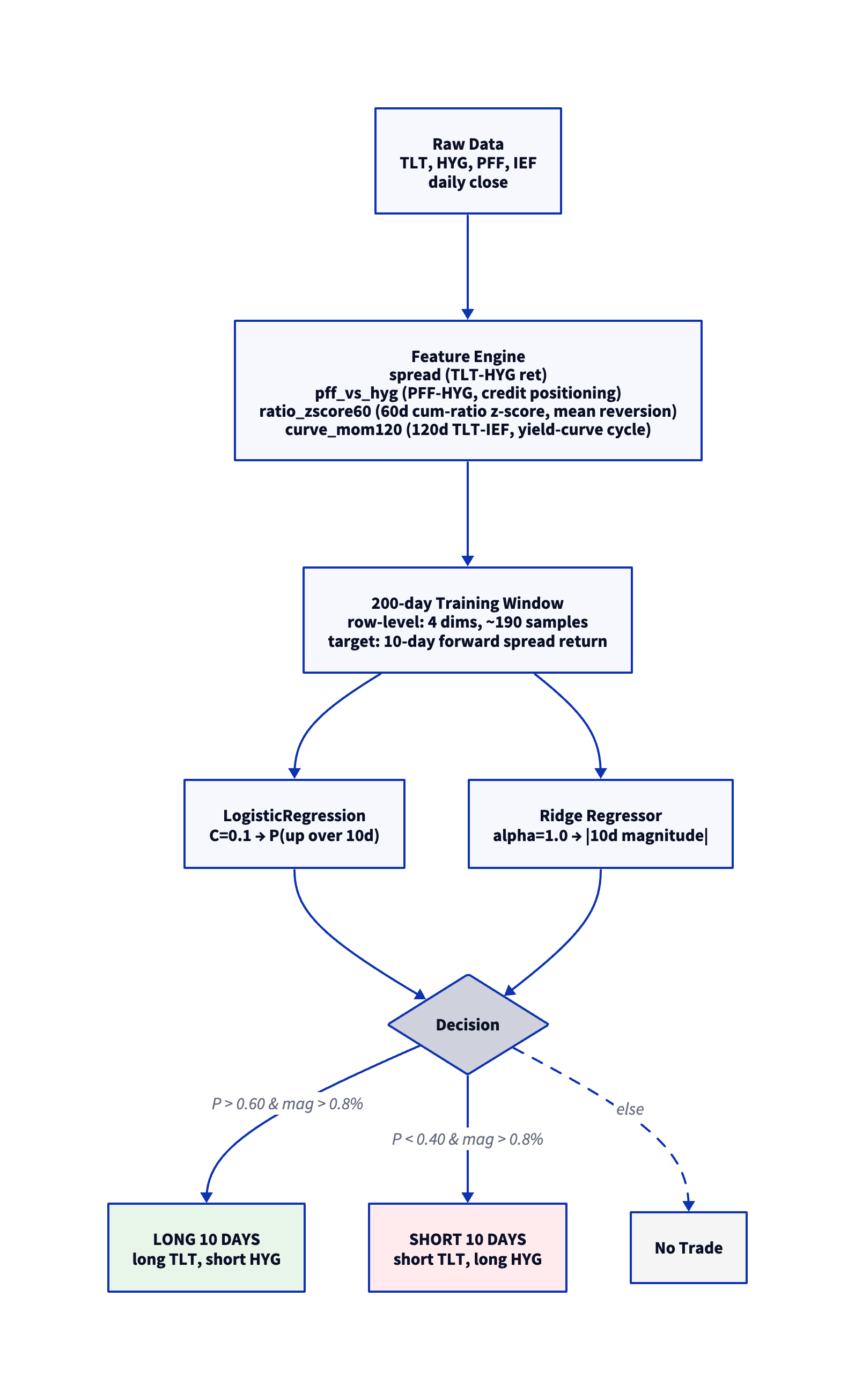
The strategy uses three signals:
Credit positioning (PFF-HYG): Preferred shares (PFF) sit between investment-grade and high-yield in the capital stack. The PFF-HYG spread is a clean read on credit-cycle positioning that leads broader credit moves by 1-2 weeks. When PFF outperforms HYG, credit risk-off is starting (TLT will rally vs HYG).
Mean reversion (60d cumulative-ratio z-score): TLT-HYG cumulative spreads have strong mean-reverting properties on multi-week scales. When the cumulative spread is multiple standard deviations from its 60-day mean, reversion typically pays.
Yield-curve cycle (120d TLT-IEF momentum): The yield-curve regime (long-end vs intermediate Treasuries) drives the broader bond market. The 120-day curve trend captures the slow-moving rate-cycle dynamic that affects TLT directly and HYG indirectly through corporate refinancing.
1.2 Why 10-Day Holds
Fixed-income macro signals operate on weekly to monthly cycles, not daily. The horizon dependence is dramatic:
Hold Period
Net Sharpe (post-10bps)
10-day
5.86
5-day
3.52
3-day
3.30
2-day
0.87
Daily
0.40
Daily and 2-day holds capture noise; 10-day holds capture the actual credit-cycle signal. This is why earlier pair-trading attempts on fixed-income often fail — they use the wrong holding period.
Enter when the model predicts a 10-day spread move exceeding 0.8%. Hold for 10 trading days. Each entry incurs one round-trip of transaction costs for 10 days of exposure – a 70%+ reduction in cost drag vs a daily strategy.
TLT/HYG is a hedge sleeve for the commodity-cluster strategies. Drawdown correlations with the other 7 sleeves:
Pair
Drawdown Corr
vs XME/DBB (metals)
-0.14
vs GDX/GLD (gold)
-0.21
vs XLE/USO (energy)
-0.22
vs EFA/SPY (intl equity)
-0.02
vs XLF/XLY (sector rotation)
-0.06
vs LMT/RTX (defense)
+0.03
vs MTUM/USMV (factor rotation)
-0.07
Consistently negative or near-zero across all sleeves. When commodity strategies struggle (typically during deflationary or strong-USD episodes when credit rallies and Treasuries underperform), TLT/HYG tends to thrive.
7. Limitations and Risks
High dollar PnL but largest open exposure: 10-day hold periods mean the strategy is in position ~80% of the time. Capital is consistently deployed (vs daily-hold sleeves that are flat 50%+ of days).
413 trades over 6.3 years (~65/year). Statistical confidence on 68.0% accuracy with 413 trades has a 95% CI of roughly 63-72%.
Sharpe of 6.49 is suspiciously high. Selected via grid search. True out-of-sample Sharpe is likely lower; expect 3-4 in production.
Bond market regime risk: The 2020-2025 backtest captures one rate cycle (Fed cutting → Fed hiking → Fed cutting). A prolonged sideways or trendless rate regime could weaken the curve_mom120 signal.
HYG liquidity events: HYG saw extreme dislocations in March 2020 and September 2022. The strategy navigated both, but future credit events could behave differently.
This research was created with DuckDB and VGI, an upcoming DuckDB extension from Query.Farm that allows custom aggregate functions to be written in any language with an Apache Arrow implementation.